
Due to the outbreak of COVID-19, our lives have been turned upside down in 2020. Professional sports will look different in 2020, but in the last few weeks we have been given some clarity on what the MLB season will look like. There will be a total of 60 regular season games down from an originally scheduled 162. The length of the season has been one of the strengths of the MLB in the eyes of many baseball purists, as it provides a large sample size which ensures that the best teams rise to the top at the end of the season and the best players are awarded the game’s top honors at season’s end.
Why is sample size important?
Baseball and statistics have long been synonymous, which is why I have no hesitation to consistently link these two in my writing. The sample size is defined as:
“the number of trials in an experiment”
The classic example that we think of is flipping a coin. An unbiased, or unweighted, coin will have an equal probability of landing on head or tails. 50 percent chance, correct? So if we perform an “experiment” where we flip an unweighted coin four times, we would expect the coin to twice land on heads and twice on tails. (We’ll use Python throughout this post to demonstrate these experiments.)
n = 4
choices = ['heads', 'tails']
result = np.random.choice(choices, n)
print("Total Trials", n, "\nHeads:", sum(result == 'heads'), "\nProbability of Heads:", sum(result == 'heads')/n)
//
Total Trials: 4
Heads: 1
Probability of Heads: 0.25
If we rely on the results of a small experiment consisting of a sample size of four trials, we might erroneously suspect the coin of being biased towards a result of heads. In practice, it takes more sampling to unlock the exact (if there is such a thing) probability of a result. What if we perform our coin flip experiment again, this time with ten trials:
Total Trials: 10
Heads: 4
Probability of Heads: 0.4
And then with 100 trials?
Total Trials: 100
Heads: 60
Probability of Heads: 0.6
What we see is that even at 100 trials there is a chance that our experiment fails to reveal the true probability of the coin flipping heads. Eventually if we kept flipping coins, the true probability of 50 percent would be inescapably clear. This should help explain why the game of baseball is favored by statistician’s over other games. The larger our sample size (i.e. more games, pitches, plate appearances etc.) the better understanding we have about the game because in the long run the truth shall be revealed!
Power
So we’ve established that sample size is important and has a significant impact on our view of the world and we know that the more trials we conduct in an experiment the more certain we are of the outcome. We clearly can’t have an infinite number of trials though, so how do we determine the sufficient amount of trials to conduct? This brings us to statistical power, a measure of the confidence of an experiment.
\[\beta = \Phi\left(\frac{|\mu_t-\mu_c|\sqrt{N}}{2\sigma}-\Phi^{-1}\left(1-\frac{\alpha}{2}\right)\right)\]Power is represented by \(\beta\) and the \(\Phi(\bullet)\) is the normal cumulative distribution function with the effect size being represented by \(\mid\mu_t-\mu_c\mid\), \(\alpha\) being the desired level of statistical significance which is typically 0.05, and N representing the sample size. Let’s rely on the statsmodel Python module for our power calculations. Before we get back to baseball, let’s use our coin-flipping example to demonstrate how this works.
Suppose we have a coin that we suspect is biased to flipping tails 40 percent of the time. If we were to conduct an experiment to prove this suspicion, how many times would we need to flip the coin? The power solver in statsmodels allows us to specify our desired power and it will compute the number of samples needed. Here, we’re going to aim for a power of 0.8 and an \(\alpha\) of 0.05 which are both pretty standard in scientific research. We’ll also need to specify the effect size, which will be the difference between the an unbiased coin (\(\mu_c=0.5\)) and the supposed biased coin (\(\mu_t=0.4\)).
from statsmodels.stats.power import  tt_ind_solve_power
mu_t, mu_c = 0.5, 0.4
effect_size = mu_t - mu_c
N, alpha, power = 1000, 0.05, 0.8
Ncalc = tt_ind_solve_power(effect_size=effect_size, power=power, nobs1=None, alpha=alpha, ratio=1.0)
print(Ncalc)
//
1570.733066331529
Our power calculation tells us that we need to perform 1,570 coin flips to satisfy these constraints. In English, this means that if we want 80% of our experiments to detect an effect change of 0.1 with 95% confidence, then we must have a sample size of at least 1,570.
Variance of outcomes
Power of 0.8 is a high bar to set for a lot of experiments. In actuality there are compromises that need to be made. Even using the toy example of flipping a coin. If I ask my kids to conduct this coin flipping experiment, I bet they could stay focused on it for 100, maybe 200 coin flips. But 1,570? I doubt it. The outcome of the experiment is subject then to higher variance which means the result is more likely to be wrong (i.e. less confident).
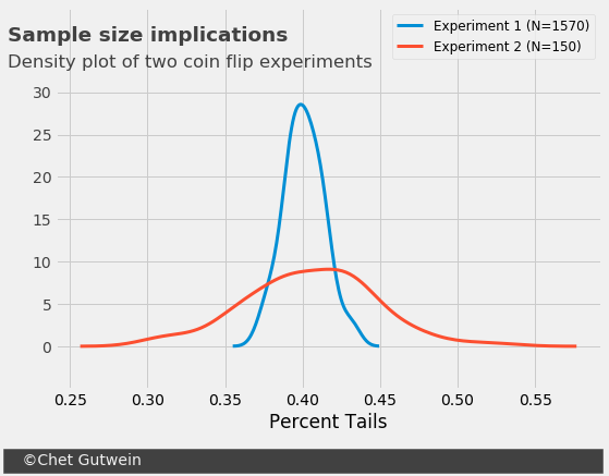
We can test this by simulating the experiment many times and seeing how different the results are. We’ll replicate the experiment using numpy 100 times each as follows:
- Experiment 1: Biased coin, 1,570 samples
- Experiment 2: Biased coin, 150 samples
from scipy import stats
N_1 = 1570
results_1 = np.empty([1,100])
for i in range(100):
    temp_result = np.random.choice(choices, N_1, p=[mu_c, 1-mu_c])
    results_1[0,i] =sum(temp_result == 'heads')/N_1
print("Experiment 1:",results_1.mean(), results_1.std(), results_1.var())

N_2 = 150
results_2 = np.empty([1,100])
for i in range(100):
    temp_result = np.random.choice(choices, N_2, p=[mu_c, 1-mu_c])
    results_2[0,i] =sum(temp_result == 'heads')/N_2
print("Experiment 2:",results_2.mean(), results_2.std(), results_2.var())
//
Experiment 1: 0.4009044585987261 0.012835044474719165 0.00016473836666801897
Experiment 2: 0.40493333333333337 0.04107034615550901 0.0016867733333333337
The mean results of both experiments is essentially identical, with heads at 40.1% for Experiment 1 and 40.5% for Experiment 2. But the variance for Experiment 2 is almost three times what it is for Experiment 1. Typically we would set a confidence interval of \(2\sigma\), or two standard deviations, from the mean. This gives us the following conclusion from the two experiments:
- Experiment 1: True probability of heads is between 37.5% and 42.7%
- Experiment 2: True probability of heads is between 32.3% and 48.7%
Okay now we can get back to baseball…
What to expect in MLB’s short season?
So why did we spend so much time talking about flipping a coin? Determining the winner of a baseball game is the same thing. We’re going to run another simulation, but it’s not going to model a baseball season with a sophisticated algorithm that includes player’s season histories or even pitching match-ups. We’re going to model games as if they’re coin flips and we’ll use Dan Szymborski’s ZIPS projections for 2020 to establish the bias of our coins. Since I write for Purple Row and I’m a Rockies fan, we’ll use the Rockies as our case example.
To preface our simulation of the Rockies season, we need to establish a wins target for this team. They are very, very unlikely to win the NL West division, although with the shorter season this does become somewhat less unlikely. So, a Wild Card birth to the post-season is their path to the playoffs. For a 162-game season, it typically takes around 90 wins. If we prorate this for a 60 game season we’re looking at 33.3 wins. To be safe, we’ll target 34 wins. The ZiPS latest projection has the Rockies expected winning percentage at 0.433. So the Rockies are now a biased coin that flips heads 43.3 percent of the time. Now we’ll once again run two separate simulations:
- Simulation 1: 162-game season (100 replications)
- Simulation 2: 60-game season (100 replications)
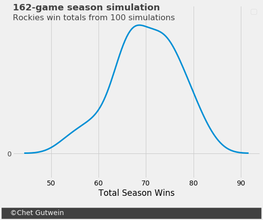
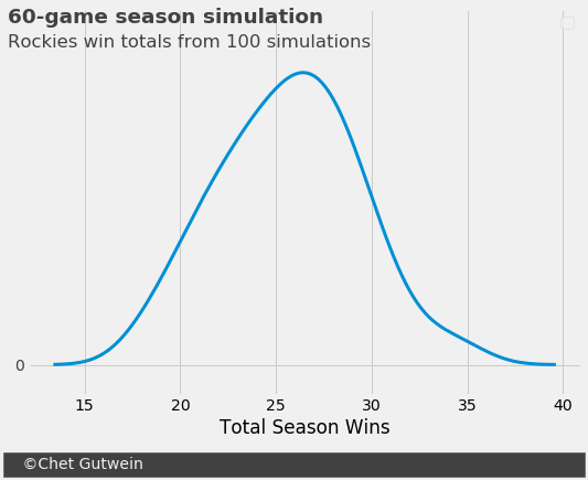
For a 162-game season, the Rockies have a less than 0.1 percent chance of winning more than 83 games. They are not a playoff team in a 162-game season unless they massively overperform ZiPS, I don’t care what Dick Monfort says. But in a 60-game season, they have about a 1.0 percent chance of making the playoffs if 34 games is an accurate wins benchmark. This might not seem like much, but going from a “snowball’s chance in hell” to 1.0 percent is a very significant change. The shorter schedule will more greatly affect the playoff chances for teams with a projected winning percentage around 0.500.
The charts in this post were created in python. Supporting documentation can be found here.